WiSTL x-t Diagram

WiSTL
Home

College of

Engineering

	Wisconsin
	Institute for
	Nuclear
	Safety

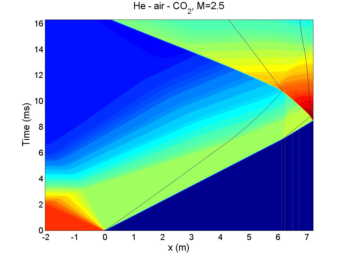
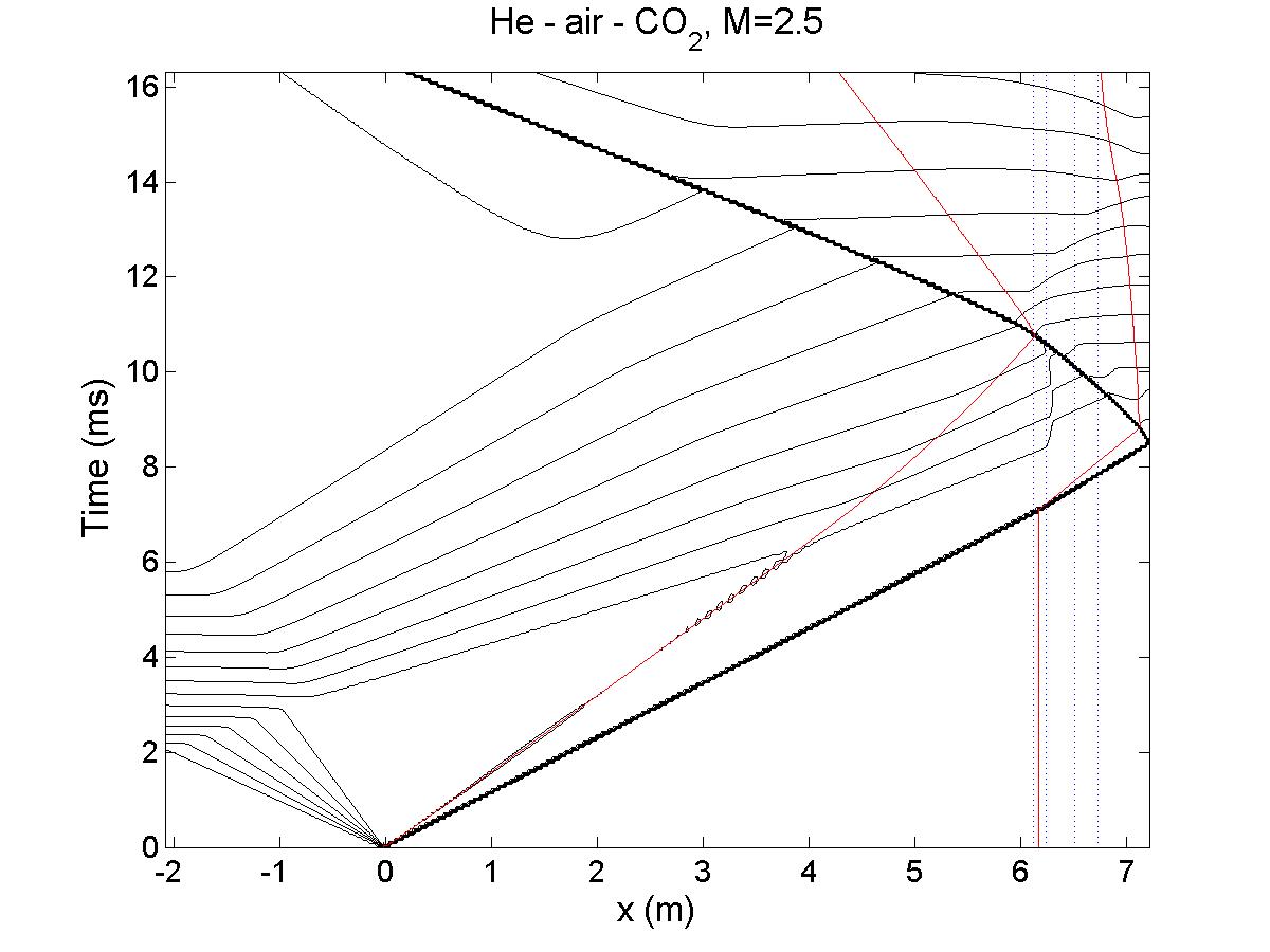
x-t Diagram Tools

An x-t diagram can be a useful experimental design tool for shock tube experiments as it details shock and rarefaction waves propagating in the tube. A common diagnostic in WiSTL experiments is the imaging of a shocked interface in the test section. The timing issues associated with the illumination of the interface and/or the camera shutter control may be calculated analytically, however, the x-t diagram provides additional information, such as, when the reflected shock off the bottom of the shock tube comes back and interacts with the interface, and when (and if) the rarefaction from the driver catches up to the shock wave before it interacts with the interface.


Fig. 1 - Color Plot	Fig. 2 - Contour Plot

Click plot to enlarge.

The following three files can be used to create the color and contour plots shown in Figs. 1 and 2:

xt.exe - a 2nd order, Muscl-Hancock-Method finite volume code with an exact Riemann solver (win32 binary, 661 kB)
param.in - the input file for xt.exe (ascii, 1 kB)
xt.m - a Matlab script for creating the diagrams (ascii, 3 kB)

Note: this program generates 30 MB of data files. To begin, the program xt.exe is run at a DOS command line. The program reads in the user input located in the file "param.in" and creates a number of data files. The Matlab script "xt.m" reads in the data files (e.g. pressure for the waves shown in Figs. 1 and 2) and generates the plots.

If you can regenerate Figs. 1 and 2 you are ready to start modifying the input and generating new x-t diagrams. You will need to modify the file "param.in" to suit your shock tube and gas combinations. Lines 4-6 from the file are the desired length of the shock tube and locations of the diaphragm and interface. Lines 7-21 are the appropriate parameters for the three gases, gas 1 is the test gas (occupying one end of the shock tube), gas 2 is the driven gas (occupying the space between the interface and diaphragm), and gas 3 is the driver gas. Line 22 is a parameter for determining the slope vectors (if you don't know what this means, don't worry, just leave it as is, if you would like more information, see Ch. 13 and 14 of "Riemann Solvers and Numerical Methods for Fluid Dynamics," by E.F. Toro, Springer, 1999.)

Lines 1-3 require a little more explanation. The variable on line 1 is "nsteps", the larger the number, the larger the datafiles, and the prettier the picture. Line 2 is "deltat" and is calculated according to the following:

deltat	= 2	Ldriver - Ldiaph
		W*nsteps

where W is the initial shock wave speed. In the sample input file, the shock wave is M=2.5 in air, W=955 m/s and can be obtained using the Gas Dynamics Calculator. Therefore:

deltat	= 2	9.298 - 2.08	= 6 x 10^-5 s
		955 * 250

This is a good starting point for deltat, if you decide you want to watch the waves progress further in time then increase the deltat. Line 3 sets a stability criteria for the code and the maximum wave speed is the sum of the particle velocity and sound speed in region 2, also obtained using the Gas Dynamics Calculator.

A couple of notes about the Matlab script. The two red lines in the contour plot track the location of the diaphragm and the interface while the dashed lines are imaging window locations. The number of colors in the color plot may be increased from 64 to a higher value (128, 256, etc.) at the expense of the script taking more time to run. The appearance of the contour plot may be enhanced by decreasing or increasing the number of contour levels from the default value of 20.

Department of Engineering Physics | UW Home